Logistic Regression in Machine Learning using Python

In statistics logistic regression is used to model the probability of a certain class or event. I will be focusing more on the basics and implementation of the model, and not go too deep into the math part in this post.

Logistic regression is similar to linear regression because both of these involve estimating the values of parameters used in the prediction equation based on the given training data. Linear regression predicts the value of some continuous, dependent variable. Whereas logistic regression predicts the probability of an event or class that is dependent on other factors. Thus the output of logistic regression always lies between 0 and 1. Because of this property it is commonly used for classification purpose.

Logistic Model

Consider a model with features x1, x2, x3 … xn. Let the binary output be denoted by Y, that can take the values 0 or 1. Let p be the probability of Y = 1, we can denote it as p = P(Y=1).

The mathematical relationship between these variables can be denoted as:

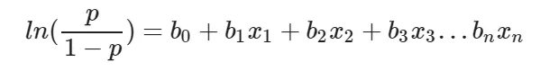
Here the term p/(1−p) is known as the odds and denotes the likelihood of the event taking place. Thus ln(p/(1−p)) is known as the log odds and is simply used to map the probability that lies between 0 and 1 to a range between (−∞,+∞). The terms b0, b1, b2… are parameters (or weights) that we will estimate during training.

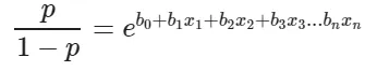
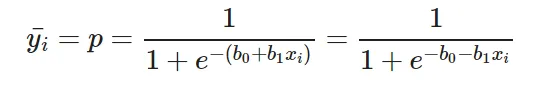
So this is just the basic math behind what we are going to do. We are interested in the probability p in this equation. So we simplify the equation to obtain the value of p:

1. The log term ln on the LHS can be removed by raising the RHS as a power of e:

2. Now we can easily simplify to obtain the value of p:

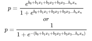
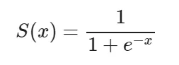
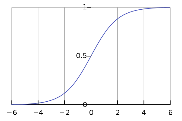
This actually turns out to be the equation of the Sigmoid Function which is widely used in other machine learning applications. The Sigmoid Function is given by:

Now we will be using the above derived equation to make our predictions. Before that we will train our model to obtain the values of our parameters b0, b1, b2… that result in least error. This is where the error or loss function comes in.

Loss Function

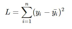
The loss is basically the error in our predicted value. In other words it is a difference between our predicted value and the actual value. We will be using the L2 Loss Function to calculate the error. Theoretically you can use any function to calculate the error. This function can be broken down as:

1. Let the actual value be yᵢ. Let the value predicted using our model be denoted as ȳᵢ. Find the difference between the actual and predicted value.

2. Square this difference.

3. Find the sum across all the values in training data.

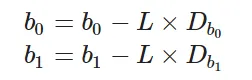
Now that we have the error, we need to update the values of our parameters to minimize this error. This is where the “learning” actually happens, since our model is updating itself based on it’s previous output to obtain a more accurate output in the next step. Hence with each iteration our model becomes more and more accurate. We will be using the Gradient Descent Algorithm to estimate our parameters. Another commonly used algorithm is the Maximum Likelihood Estimation.

The Gradient Descent Algorithm

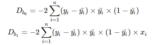
You might know that the partial derivative of a function at it’s minimum value is equal to 0. So gradient descent basically uses this concept to estimate the parameters or weights of our model by minimizing the loss function. Click here for a more detailed explanation on how gradient descent works. For simplicity, for the rest of this tutorial let us assume that our output depends only on a single feature x. So we can rewrite our equation as:

Thus we need to estimate the values of weights b0 and b1 using our given training data.

1. Initially let b0=0 and b1=0. Let L be the learning rate. The learning rate controls by how much the values of b0 and b1 are updated at each step in the learning process. Here let L=0.001.

2. Calculate the partial derivative with respect to b0 and b1. The value of the partial derivative will tell us how far the loss function is from it’s minimum value. It is a measure of how much our weights need to be updated to attain minimum or ideally 0 error. In case you have more than one feature, you need to calculate the partial derivative for each weight b0, b1 … bn where n is the number of features. For a detailed explanation on the math behind calculating the partial derivatives, check out my video.

3. Next we update the values of b0 and b1:

4. We repeat this process until our loss function is a very small value or ideally reaches 0 (meaning no errors and 100% accuracy). The number of times we repeat this learning process is known as iterations or epochs.

Implementing the Model

Import the necessary libraries and download the data set here. The data was taken from kaggle and describes information about a product being purchased through an advertisement on social media. We will be predicting the value of Purchased and consider a single feature, Age to predict the values of Purchased. You can have multiple features as well.

# Importing libraries
import numpy as np
import pandas as pd
import matplotlib.pyplot as plt
from sklearn.model_selection import train_test_split
from math import exp
plt.rcParams["figure.figsize"] = (10, 6)

# Download the dataset
# Source of dataset - https://www.kaggle.com/rakeshrau/social-network-ads
# !wget "https://drive.google.com/uc?id=15WAD9_4CpUK6EWmgWVXU8YMnyYLKQvW8&export=download" -O data.csv -q

# Load the data
data = pd.read_csv("data.csv")
data.head()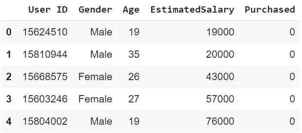

# Visualizing the dataset
plt.scatter(data['Age'], data['Purchased'])
plt.show()

# Divide the data to training set and test set
X_train, X_test, y_train, y_test = train_test_split(data['Age'], data['Purchased'], test_size=0.20)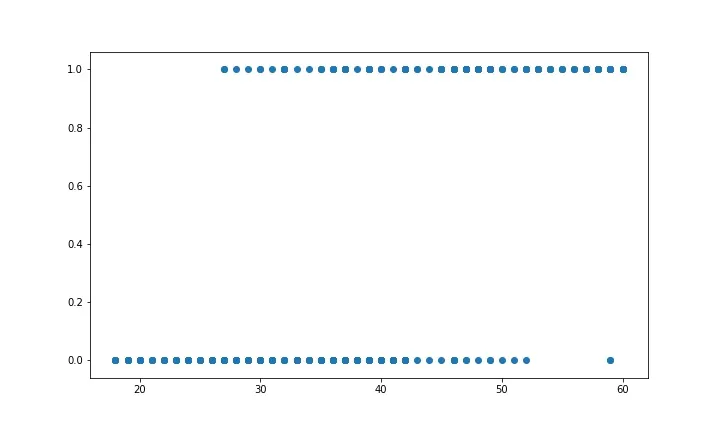

We need to normalize our training data, and shift the mean to the origin. This is important to get accurate results because of the nature of the logistic equation. This is done by the normalize method. The predict method simply plugs in the value of the weights into the logistic model equation and returns the result. This returned value is the required probability.

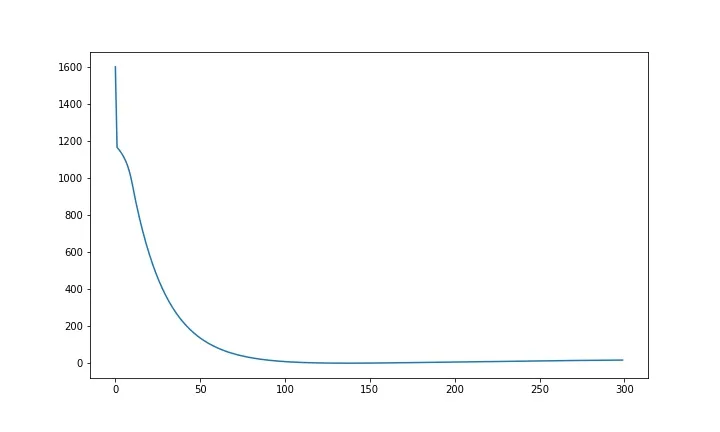
The model is trained for 300 epochs or iterations. The partial derivatives are calculated at each iterations and the weights are updated. You can even calculate the loss at each step and see how it approaches zero with each step.

# Creating the logistic regression model

# Helper function to normalize data
def normalize(X):
    return X - X.mean()

# Method to make predictions
def predict(X, b0, b1):
    return np.array([1 / (1 + exp(-1*b0 + -1*b1*x)) for x in X])

# Method to train the model
def logistic_regression(X, Y):

    X = normalize(X)

    # Initializing variables
    b0 = 0
    b1 = 0
    L = 0.001
    epochs = 300

    for epoch in range(epochs):
        y_pred = predict(X, b0, b1)
        D_b0 = -2 * sum((Y - y_pred) * y_pred * (1 - y_pred))  # Derivative of loss wrt b0
        D_b1 = -2 * sum(X * (Y - y_pred) * y_pred * (1 - y_pred))  # Derivative of loss wrt b1
        # Update b0 and b1
        b0 = b0 - L * D_b0
        b1 = b1 - L * D_b1
    
    return b0, b1

Since the prediction equation return a probability, we need to convert it into a binary value to be able to make classifications. To do this, we select a threshold, say 0.5 and all predicted values above 0.5 will be treated as 1 and everything else will be 0. You can choose a suitable threshold depending on the problem you are solving.

Here for each value of Age in the testing data, we predict if the product was purchased or not and plot the graph. The accuracy can be calculated by checking how many correct predictions we made and dividing it by the total number of test cases. Our accuracy seems to be 85%.

# Training the model
b0, b1 = logistic_regression(X_train, y_train)

# Making predictions
X_test_norm = normalize(X_test)
y_pred = predict(X_test_norm, b0, b1)
y_pred = [1 if p >= 0.5 else 0 for p in y_pred]

plt.clf()
plt.scatter(X_test, y_test)
plt.scatter(X_test, y_pred, c="red")
plt.show()

# The accuracy
accuracy = 0
for i in range(len(y_pred)):
    if y_pred[i] == y_test.iloc[i]:
        accuracy += 1
print(f"Accuracy = {accuracy / len(y_pred)}")

Accuracy = 0.85

Implementing using Sklearn

The library sklearn can be used to perform logistic regression in a few lines as shown using the LogisticRegression class. It also supports multiple features. It requires the input values to be in a specific format hence they have been reshaped before training using the fit method.

The accuracy using this is 86.25%, which is very close to the accuracy of our model that we implemented from scratch!

# Making predictions using scikit learn
from sklearn.linear_model import LogisticRegression

# Create an instance and fit the model 
lr_model = LogisticRegression()
lr_model.fit(X_train.values.reshape(-1, 1), y_train.values.reshape(-1, 1))

# Making predictions
y_pred_sk = lr_model.predict(X_test.values.reshape(-1, 1))

plt.clf()
plt.scatter(X_test, y_test)
plt.scatter(X_test, y_pred_sk, c="red")
plt.show()

# Accuracy
print(f"Accuracy = {lr_model.score(X_test.values.reshape(-1, 1), y_test.values.reshape(-1, 1))}")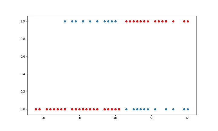

Accuracy = 0.8625

Thus we have implemented a seemingly complicated algorithm easily using python from scratch and also compared it with a standard model in sklearn that does the same. I think the most crucial part here is the gradient descent algorithm, and learning how to the weights are updated at each step. Once you have learned this basic concept, then you will be able to estimate parameters for any function.